When you work with an enormous Excel spreadsheet (spreadsheet), many columns and rows are duplicated. It is necessary to do a lot of work to organize the columns and rows, as duplicate data is an annoyance that no one would like to endure.
In Excel, you can gather data, alter analysis, analyze and convert data any way you want. Identifying duplicate data is challenging, but in the same way, it’s not difficult to do. We’ve developed several methods that allow you to use a formula for identifying duplicates within Excel. After identifying duplicates, you’re free to use whatever way you like.
Utilizing Formula to find Duplicates Excel Excel
Using Excel formulas makes it possible to detect duplicate values without difficulty. Once you’ve learned how to utilize procedures, you’ll also learn to use different recipes, including CONCATENATE.
Find duplicates using Excel.
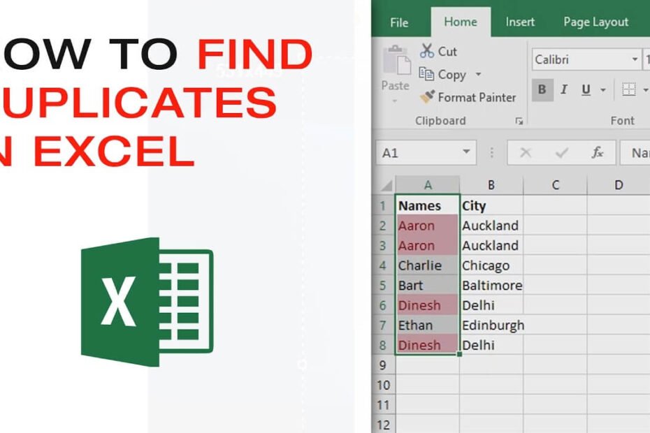
If you want to look for duplicates so that you’ll be able to decide if you wish to remove them, the ideal option is to draw attention to any duplicate content with conditional formatting.
Choose the information you wish to look for duplicate data. Choose the Conditional Formatting tab from the home tab, Highlight Cell Rule Rules and Duplicate values.
On the Conditional Formatting window, which opens in the middle, select the drop-down menu under Format to choose the colour scheme you prefer to highlight duplicates. After that, click Done. (Tip to choose a higher contrast scheme of colour, like Fill with light red to make it easier to read.)
Now you can review the duplicates and decide if you want to remove any redundant data.
What is the COUNTIF Function within Excel
If you’d like to find the number of times the same value occurs in a data set, use the COUNTIF feature in Excel. COUNTIF is a tool that can count cells with a particular number of deals, cells with more or less than a certain value, and cells with an amount within a specific range. In this post, we’ll demonstrate how to use COUNTIF to detect duplicates within the dataset.
To use COUNTIF in finding duplicates, it is necessary to be able to organize your data on a spreadsheet with every value placed in its cell. Then, you can utilize the COUNTIF function to calculate the number of times each value is present in the data set. To accomplish this, type the Formula below into the blank cell.
=COUNTIF(A1:A10,A1)
The Formula counts the total number of cells within the A1:A10 range with the Formula in A1. Using the Formula for other cells within this column is then possible to determine how many times each value appears within the data set.
It is also possible to use the COUNTIF function to figure out the number of instances an item appears in a set of data that is greater or below a particular amount. If, for example, you were looking to determine how often a given value is found in a set higher than 5, you’d apply the Formula below:
=COUNTIF(A1:A10,”>5″)
The Formula is used to count the number of cells within the A1:A10 range with an amount greater than five. It is then possible to move the Formula downwards into the remaining cells of this column to determine how many times every value is present within the dataset.
Additionally, you can utilize the COUNTIF formula to determine the number of times an item appears in a data set between two figures. In the example above, if you want to know the number of times a particular value is found in a set that falls between five to 10, you’d apply the Formula below:
=COUNTIF(A1:A10,”>5
How to Remove Duplicates from Excel Using PowerQuery
Power Query is an innovative Excel instrument used for ETL (Extract, Transform, and load). Power Query allows you to collect data from various sources and use transformations. It offers a data cleaning process to alter it to your requirements.
Take these steps to get rid of duplicates with Power Query.
Step 1: Make tables by drawing rows and choosing Insert Table. You can also hit CTRL+T and create tables. Make sure that the table is a header.
Step 2: Click on the Data tab. In the Get & Transform Data, choose the option from Table or Range.
3: The Power Query Editor is opened, from where you are able to perform the required transforms.
4. Click Home – Remove Rows Eliminate duplicates.
5: In the Settings tab, you will see the message “Remove duplicates.’
6: Following this reply, click Home to Close & Load.
7. receive the table, with duplicates eliminated and a new sheet.
By using the filter feature
The Filter function in Excel Online can also be employed to find and remove duplicates swiftly. To use this feature, you must first choose the cells you want to find duplicates. Next, go to the Data tab of the ribbon and choose the filter option. The drop-down arrows will be added to the column headers in the opportunity. Select the drop-down arrow on the column where you wish to look for duplicates, then select the option to filter by colour. Select the colour to highlight the duplicates, then click OK. Then, you will see only duplicate entries within the list you erase.
The Best Way to Deal with Errors as well as Inconsistencies
The inconsistencies in your data could affect the process of comparison. Here are four suggestions to resolve inconsistencies
Look for differences in different data types, like mixing numbers and text within the same column.
Ensure the same formatting style is utilized when formatting dates, numbers, and other types of data.
Check your records for errors or missing entries, then correct them when necessary.
Use standard abbreviations and consistent names within your set of data.
What is it that you mean by highlighting duplicates? And how can this do using Excel?
The value of a duplicate is found several times within an array of data. The copies are highlighted to simplify the data. Additionally, the highlight feature makes it possible for the user to look at every duplicated value and choose whether or not to keep the duplicate.
How to search for duplicates and highlight them in Excel are as follows:
a. Choose the area in which duplicates will be identified and highlighted.
B. Select to open the “conditional formatting” drop-down from the Home tab in Excel. Choose “duplicate values” from “highlight cells rules.”
C. The”Values that are duplicated” box appears. Choose the formatting you require among the options within the “values with” box. Select “Ok.”
The duplicates that fall within the area are identified and highlighted using the colour chosen in Step C.
SUBMITTING THINKS
This is the final part of this tutorial on identifying duplicates in Excel. I’ve provided all the most popular ways for users to locate copies within Excel. These methods are guaranteed to be useful and sufficient for most users.
Check out our free Excel resource section if you need more comprehensive information about Excel capabilities and functions.
If you want to gain a deeper understanding and practice using Excel check out our Excel courses here.